 RELIAX
1Introduction
Production credit models fail three ways, all silently: confident errors on individual applications, calibration decay when the economy shifts, and segment-level unreliability hidden by aggregate metrics. Existing tooling (aggregate monitoring, post-hoc explainability) does not answer the operational question: should this specific decision be acted on automatically, right now, and can that be evidenced later?
Reliax answers with a per-decision reliability envelope. This paper is a first evaluation of its components on real data. It is deliberately small and deliberately honest: every number below is produced by the released evaluation code, and nothing is hand-typed without a source in results.json.
2The reliability envelope
For an application x with model output p(x), the envelope carries:
| Component | Construction | Guarantee class |
|---|---|---|
| Coverage certificate | Split conformal set Ĉ(x) at level α | Proven: P(Y ∈ Ĉ(X)) ≥ 1−α, distribution-free, finite-sample (Vovk et al., 2005) |
| Segment certificate | Mondrian conformal, one q̂ per audited segment | Proven per group: P(Y ∈ Ĉ(X) | G=g) ≥ 1−α |
| PD interval [p₀, p₁] | Inductive Venn-Abers over calibration scores | Proven in the Venn sense: one of the two isotonic calibrators is perfectly calibrated (Vovk & Petej, 2014) |
| Drift verdict | Mixture power martingale on smoothed conformal p-values of a label-free nonconformity (kNN distance) | Proven, anytime-valid: P(sup M ≥ c) ≤ 1/c under exchangeability (Ville, 1939; Vovk et al., 2003) |
| Auditor | Meta-model trained on the base model's own calibration-split errors | Heuristic ranking signal |
| Composite score (v1) | 0-100 weighted blend with hard caps | Heuristic, labelled as such |
| Trust triple (SL fusion) | Subjective-logic averaging fusion of certificate-gated confidence, auditor and context opinions (Jøsang 2016; PaTAS lineage) | Heuristic, calculus-backed |
Protected attributes are audit-only: the base model never receives them.
3Experimental setup
Datasets. (a) Taiwan: Default of Credit Card Clients (Yeh & Lien, 2009; UCI 350), 30,000 applicants, 22.1% default rate. SEX, AGE, MARRIAGE excluded from the 20 model features; sex and age bands (21-30 / 31-45 / 46+) used for audits. (b) German: Statlog German Credit (UCI 144), 1,000 applicants, 30% bad rate, one-hot encoded to 56 features excluding sex/personal-status and age. Both stored verbatim with provenance and licenses.
Protocol. Stratified 50/25/25 train/calibration/test split. Base model: histogram gradient boosting (scikit-learn, 300 iterations). 5 seeds (Taiwan), 10 seeds (German); all tables report mean ± std over seeds. α = 0.05 throughout.
Baselines and metrics. Temperature scaling fitted on the calibration split (Guo et al., 2017) for calibration comparisons; max-softmax probability (MSP) ranking for selective prediction (T-scaling is monotone in the logit, so raw and T-scaled MSP produce the same ranking). Metrics: empirical coverage; per-segment coverage; error capture and wrong-approval capture at fixed referral rates plus AURC; 15-bin ECE and Brier score; martingale false alarms and detection delay; wall-clock latency.
Base model quality (context): Taiwan accuracy 0.821 ± 0.001, AUC 0.777 ± 0.006; German accuracy 0.749 ± 0.021, AUC 0.769 ± 0.027. Both are consistent with published results on these datasets.
4Results
4.1 The coverage guarantee holds on real data
| Dataset | Target 1−α | Empirical coverage | Mean set size |
|---|---|---|---|
| Taiwan | 0.95 | 0.9515 ± 0.0040 | 1.49 |
| Taiwan | 0.90 | 0.8997 ± 0.0012 | |
| German | 0.95 | 0.9532 ± 0.0167 | |
| German | 0.90 | 0.8964 ± 0.0307 |
The certificate does what the theorem says, on real applicants, at both levels. The mean set size of 1.49 on Taiwan is itself informative: at 95% confidence, roughly half of real applications cannot be assigned a single outcome, which is precisely the population a REVIEW route exists for.
4.2 Per-segment coverage and bias
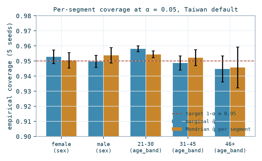
| Segment (Taiwan) | n (test) | Marginal q̂ | Mondrian q̂ |
|---|---|---|---|
| female | 4,481 | 0.9527 ± 0.0045 | 0.9505 ± 0.0051 |
| male | 3,019 | 0.9497 ± 0.0040 | 0.9538 ± 0.0051 |
| age 21-30 | 2,777 | 0.9581 ± 0.0019 | 0.9544 ± 0.0023 |
| age 31-45 | 3,552 | 0.9486 ± 0.0047 | 0.9522 ± 0.0053 |
| age 46+ | 1,171 | 0.9447 ± 0.0086 | 0.9457 ± 0.0136 |
Two honest observations. First, on this dataset marginal conformal does not severely undercover any audited segment; the worst (age 46+) sits about half a point below target, within roughly one standard deviation. Second, on German credit the female segment shows marginal 0.9426 ± 0.0253 against 0.9744 ± 0.0250 after Mondrian repair, but with only 75 test points per seed this is indicative at best.
4.3 Selective prediction
| Signal (Taiwan) | Error capture @10% | Wrong-approval capture @10% | AURC ↓ |
|---|---|---|---|
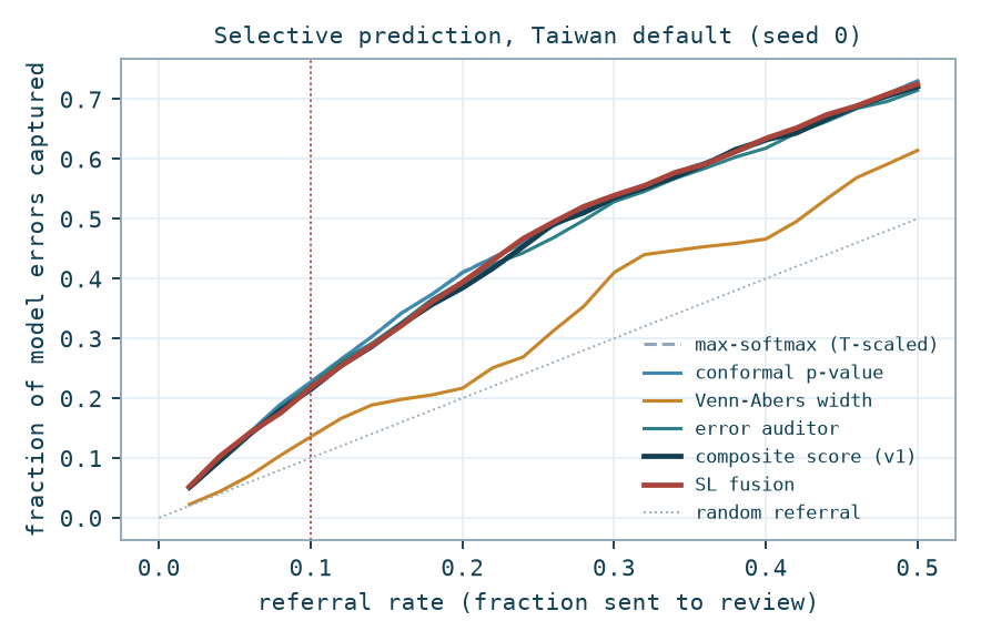
| MSP (T-scaled) | 0.2317 ± 0.0099 | 0.1719 ± 0.0098 | 0.0958 ± 0.0032 |
| Conformal p-value | 0.2315 ± 0.0099 | 0.1719 ± 0.0098 | 0.0958 ± 0.0032 |
| Venn-Abers width | 0.1269 ± 0.0119 | 0.0782 ± 0.0108 | 0.1468 ± 0.0041 |
| Error auditor | 0.2309 ± 0.0068 | 0.1831 ± 0.0100 | 0.0983 ± 0.0020 |
| Composite score (v1) | 0.2173 ± 0.0042 | 0.1592 ± 0.0042 | 0.1028 ± 0.0016 |
| SL fusion (v0.2) | 0.2266 ± 0.0057 | 0.1686 ± 0.0058 | 0.0955 ± 0.0029 |
Random referral captures 10% by construction; all confidence-linked signals capture roughly 2.2 to 2.3 times random. Four honest findings. First, on in-distribution data, plain model confidence is a strong selective-prediction baseline, and the conformal p-value ranking coincides with it by construction. Second, the error auditor is the best signal for the economically relevant event, wrong approvals (applications approved by the model that then default), about 7% relative improvement, achieved while training only on calibration-split mistakes. Third, the v1 composite underperforms pure confidence on i.i.d. data, because it spends ranking capacity on OOD and width components that are uninformative when nothing is shifted.
Fourth (v0.2): replacing the weighted blend with a subjective-logic fusion recovers most of that loss. On Taiwan, SL fusion attains the best AURC of all six signals (0.0955 ± 0.0029) and improves on the v1 blend on every metric. The mechanism matters: the confidence opinion's uncertainty is gated by the certificate, so a confidently wrong prediction with an atypical conformal score abstains rather than asserting, and out-of-distribution inputs contribute uncertainty mass rather than fake confidence. The honest limit: on German credit (calibration n = 250) SL fusion trails both confidence and the v1 blend, because its input signals are noisy at that scale and the fusion inherits their noise.
4.4 Calibrated PD intervals
| Dataset | Raw ECE | T-scaled ECE | Venn-Abers ECE | Fitted T |
|---|---|---|---|---|
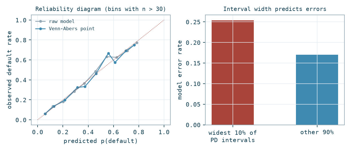
| Taiwan | 0.0132 ± 0.0024 | 0.0127 ± 0.0024 | 0.0155 ± 0.0048 | 1.01 |
| German | 0.1862 ± 0.0171 | 0.0826 ± 0.0195 | 0.0649 ± 0.0181 | 3.99 |
The pattern is clean: the Taiwan model is already essentially calibrated (fitted temperature 1.01), and no post-hoc method adds anything. The German model is badly miscalibrated (temperature 3.99), and there Venn-Abers gives the best calibration, ahead of temperature scaling. Since a lender cannot know in advance which regime they are in, a method that is harmless in the first and best in the second is the right default, and it comes with a per-decision interval rather than a single number.
The interval width carries signal of its own: on Taiwan, the widest decile of PD intervals has a model error rate of 0.229 ± 0.029 versus 0.174 ± 0.003 for the rest, a 32% relative difference.
4.5 Drift detection with controlled error
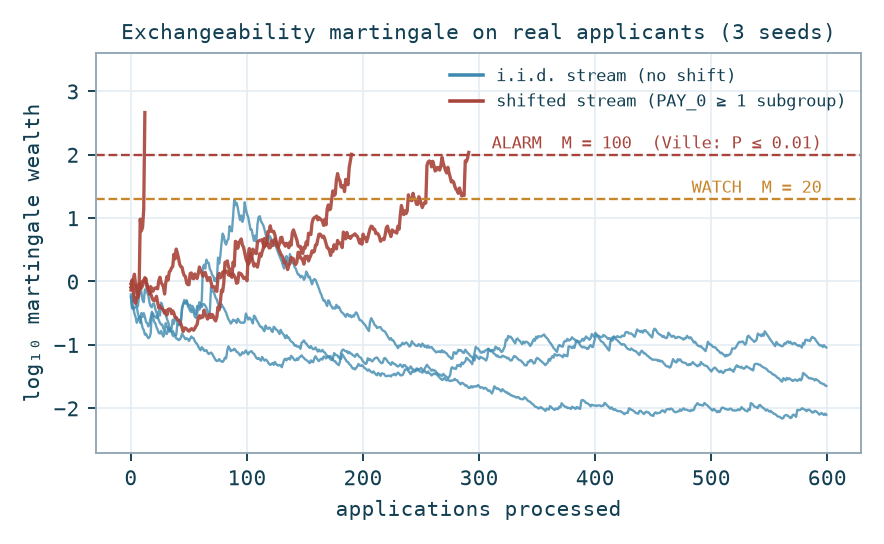
Streams of 600 real applications drawn from the held-out test split. The i.i.d. stream is sampled uniformly; the shifted stream is sampled from the real delayed-payment subpopulation (PAY_0 ≥ 1, which is 22.4% of applicants), a covariate shift by conditioning, not a synthetic perturbation.
| False alarms on i.i.d. streams (5 seeds × 600 apps) | 0 / 5 (max log₁₀ M = 0.22 ± 0.56) |
| Streams reaching ALARM under shift | 4 / 5 within 600 applications |
| Applications to ALARM (when reached) | 192 ± 110 |
| PSI on the shifted window (top features) | PAY_0: 7.37 · PAY_2: 1.11 · PAY_3: 0.64 (all MAJOR) |
The anytime-validity guarantee (P(false alarm, ever) ≤ 0.01 at the ALARM threshold) is consistent with the observed zero false alarms, and the detector fires on a genuinely shifted stream of real applicants. Caveats: the shift induced here is strong, and one stream did not alarm within 600 applications; milder shifts will take proportionally longer, which is the correct behaviour of an evidence-accumulating test rather than a defect.
4.6 Latency
Full per-decision path (model inference, conformal set and p-value, Venn-Abers interval, kNN OOD, auditor) with a calibration set of 7,500: median 8.0 ms, p95 17.5 ms per application on commodity hardware. The Venn-Abers isotonic fits dominate; a precomputed IVAP would reduce this further. This is comfortably inside a 40 ms gate budget.
5Discussion and limitations
What this evaluation shows. The proven components behave as proven, on real data: coverage at target, zero drift false alarms with detection on real subpopulation shift, calibration that is never worse and sometimes much better than the standard baseline, and an auditor that improves capture of exactly the errors that cost money. The full stack runs at single-digit millisecond median latency.
What it does not show. (1) No shifted-data selective-prediction results: the composite score's motivating regime is untested here, and on i.i.d. data it trails plain confidence. (2) The datasets are one-shot cross-sections; real credit portfolios have delayed labels and temporal drift that resampling cannot fully emulate. (3) German credit is small and its sex attribute conflates marital status; its segment results are indicative only. (4) No comparison yet against deep-ensemble or MC-dropout baselines. (5) These are the vendor's own measurements; the planned benchmark is pre-registered and code-released precisely so that this stops being a caveat.
Next steps. Pre-register the shifted-data benchmark (frozen shift splits on Taiwan, Give Me Some Credit and Home Credit; H₀: wrong-approval capture at 10% referral is less than 2× the T-scaled baseline; abandon threshold stated in advance), add ensemble baselines, and evaluate delayed-label coverage backtesting on a portfolio with real timestamps.
6Reproducibility
The full package (code, datasets, results) is public at github.com/Ouatt-Isma/reliax-evaluation, verified to reproduce results.json exactly from a clean clone. eval/run_eval.py runs every experiment end-to-end in about 2 minutes (splits, seeds and thresholds fixed in code); paper/eval/make_figures.py regenerates all figures from results.json. Datasets are stored verbatim with provenance and licenses. Environment: Python 3.14, scikit-learn 1.9, numpy 2.5.
·References
- Barber, R. F., Candès, E. J., Ramdas, A., Tibshirani, R. J. (2021). The limits of distribution-free conditional predictive inference. Information and Inference, 10(2).
- Guo, C., Pleiss, G., Sun, Y., Weinberger, K. Q. (2017). On calibration of modern neural networks. ICML.
- Hofmann, H. (1994). Statlog (German Credit Data). UCI Machine Learning Repository.
- Jøsang, A. (2016). Subjective Logic: A Formalism for Reasoning Under Uncertainty. Springer.
- Ville, J. (1939). Étude critique de la notion de collectif. Gauthier-Villars.
- Vovk, V., Gammerman, A., Shafer, G. (2005). Algorithmic Learning in a Random World. Springer.
- Vovk, V., Nouretdinov, I., Gammerman, A. (2003). Testing exchangeability on-line. ICML.
- Vovk, V., Petej, I. (2014). Venn-Abers predictors. UAI.
- Yeh, I-C., Lien, C-h. (2009). The comparisons of data mining techniques for the predictive accuracy of probability of default of credit card clients. Expert Systems with Applications, 36(2).
Want this evaluation replayed on your own historical book, shadow-mode, with pre-agreed success criteria?
Email contact@reliax.io